Finding and removing duplicate data in Excel

Finding and removing duplicate data in Excel can be a quick process. However, for many people who haven’t learnt how to do this the quick way in Excel, it can be an absolute chore.

One of the many things I love about my job is that I get to work with so many different people from all kinds of organisations. However, it doesn’t matter what industry or region I’m working in the challenges of working with large lists of data are pretty much the same.

Something I see often is the need to be able to quickly locate and remove duplicate rows of data (excellent for VLookups).  Most people just sort the data and then manually skim through the excessive lines of information trying to weed out the annoying duplicates.  This works, but boy-oh-boy it can be a time waster. Wouldn’t it be easier to have Excel quickly display the duplicates for you?  Then all you need to do is deal with them.

In this post I’m going to walk you through how to quickly locate the duplicates and then, once located, super quick ways in which to remove the duplicates.

The steps below cover:

• Locating duplicates in a single column of data
• Locating rows where the content of all cells are duplicates
• Removing the duplicate data.
  

Locating duplicates in a single column of data

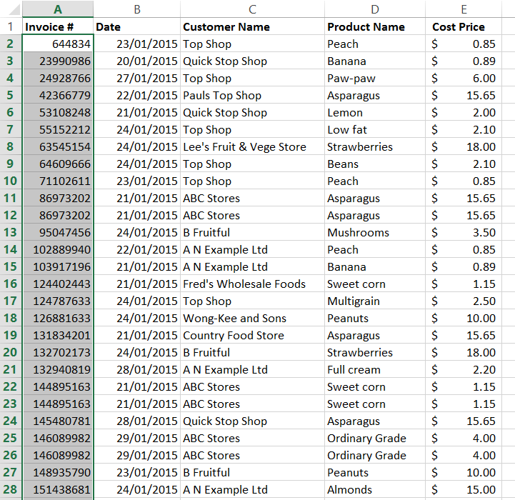
The worksheet below holds data that has been exported from an in-house system.  Unfortunately it has a number of duplicate invoice numbers in the ‘Invoice #’ column.  Using the ‘Conditional Formatting’ feature I can apply formatting to any cells with duplicate content.  All other cells will remain as they are.  This is an excellent way to very quickly identify duplicates.

1 – Select the column that holds the duplicate data.  In this case it’s the ‘Invoice #’ column.

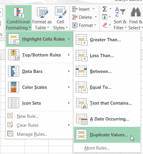
2 – From the Home tab, in the Styles group click Conditional Formatting.  A drop down menu is displayed.  Select Highlight Cell Rules from the menu.

3 – Select Duplicate Values to quickly identify duplicate or unique records.

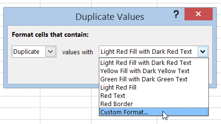
4 – The dialog box will display the condition to be matched.  In the example below the condition is ‘Duplicate’.  This setting will ensure any duplicate cells within the selected column will have the formatting applied to them.  The option box on the right displays the format that will be applied if the condition is met.  There are a range of pre-set formats available on the drop-down arrow, or if you would prefer, you can create your own by selecting Custom Format from the drop-down list.

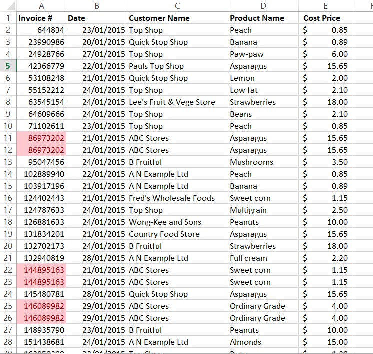
5 – Select your format options and then click OK.  All duplicates will now be formatted and easily identified.

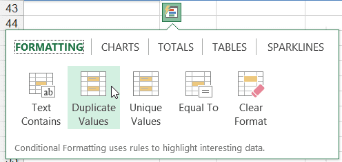
Note: You can also use the Quick Analysis tool (Excel 2013 and 2016 only) to quickly apply Conditional Formatting using default formats.  Just select the data range and then click the Quick Analysis button which will be displayed beside the selected range.  Select ‘Duplicate Values’ option.

Locating rows where the content of all cells is duplicated

In the steps above we located rows where there were only duplicate invoice numbers.  But what if you want to find duplicates where ALL of the data in a row is exactly the same as another?  For example, if you were trying to locate duplicates where the invoice number, date, customer name, product name and cost price where all exactly the same.

Here’s a quick way to do this.

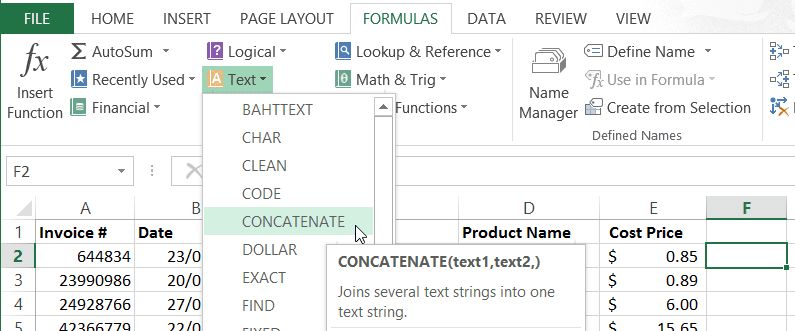
1 – The first thing to do is go to an empty cell to the right of the existing data.  Using the CONCATENATE function I’m going to pull all of the data content into this one cell.

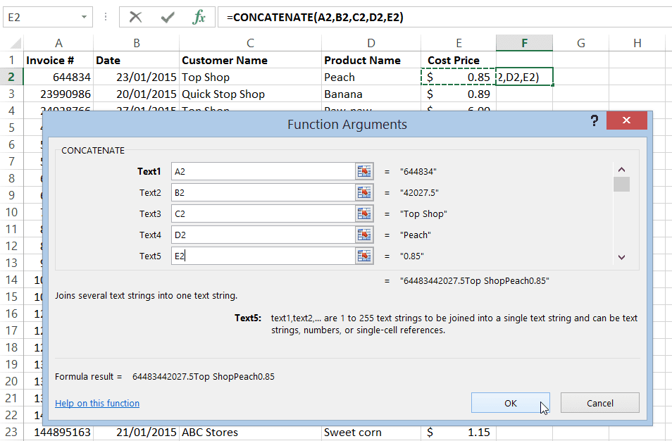
2 – In the Function Arguments dialog box enter each individual cell for the row into the Text boxes.  Note, as you enter a cell reference into one text box another will appear.  You can have up to 255 references within the function.  Once you have added all of the cells on the row click OK.  The content of all of the cells will be pulled into the one cell.

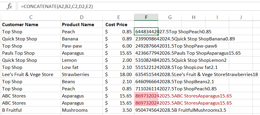
3 – Copy the function down the column and then apply to the same range of data conditional formatting to find the duplicates.  Only the cells where all cell content is the same will be formatted.

Removing duplicate rows of data

Once you have located the duplicates in most cases you will be wanting to remove them.  I see two different methods used again and again.  I’ll outline both of them.  You find your favourite.

Using Filter. If your conditional format applied a coloured background or changed the colour of the cell font you can use the Filter command to quickly filter and display only the duplicates.

1 – Select any cell in the data list and then from the Data tab click Filter.

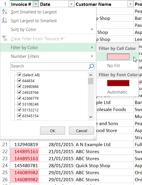
2 – Click the filter drop-down arrow on the column that is currently displaying duplicate formatting.  From the drop-down list select Filter by color and then select the cell colour or font colour depending on your conditional formats.

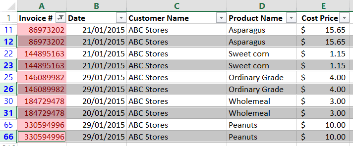
3 – Excel will filter out the unique records and only display the duplicates.

4 – Now delete the duplicate rows.  Tip: to do this quickly hold down your CTRL key and click each of the duplicate row numbers.  Once they are selected from the Home tab click Delete, Delete Sheet Rows.  All selected rows will be deleted.

5 – You will have now removed the duplicates and will only have the unique records remaining.  All formatting should now be removed as you no longer have duplicate values.

Using the ‘Remove Duplicates’ button you can have Excel quickly strip out any rows of data where duplicates are found.

1 – Select any cell in the data list and then from the Data tab select Remove Duplicates.

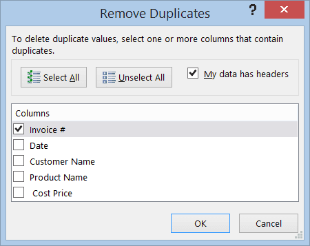
2 – Select one or more columns that contain duplicate values.

3 – Click OK.  Excel will delete any rows where duplicate values are found in the selected columns.  Please be aware that Excel will indicate how many records it has found with duplicates.  However you aren’t shown which these are prior to their removal.  If you are wanting to see them prior to removal apply conditional formatting first.

Conclusion

There is no need to spend large amounts of time locating duplicates.  Using the steps above you should be able to identify and deal with duplicates swiftly.