I think most of us will agree that error values can be helpful, and sometimes extremely unhelpful. For example, the #N/A error (Value Not Available error) is very helpful when cross-referencing two lists using the VLOOKUP function. If Excel can’t find a lookup value the #N/A error makes it very obvious.
However if you are wanting to total a range that include errors such as #N/A or #DIV/0! all of a sudden they aren’t so special any more.
Sum a range of cells that include #N/A or #DIV/0! errors
If you have tried this you will probably be totally frustrated that the SUM function just returns another #N/A value and not the required total. The same happens with the #DIV/0! (Divide by 0 error) as well.
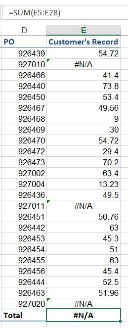
In this post I want to give you a couple of options that can be used to get past the error values and give you the range total.
Use this option if you still want to see the errors in the worksheet
Using the SUMIF function you can create a total which excludes the cells containing errors.
This option allows you to still see the #N/A errors in the Total range.
First select the cell that will hold the TOTAL. From the Formulas tab, in the Formulas group click Math & Trig. Select ‘SUMIF’ from the list.
In the ‘Range’ and ‘Sum_range’ boxes enter the range you want to total. In the ‘Criteria’ range enter “<>#N/A” and then click OK.
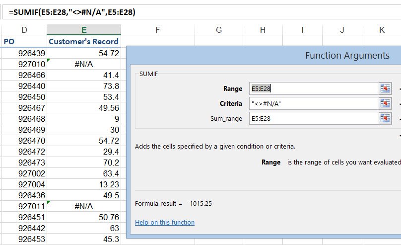
The arguments you have just entered perform the following tasks:
The ‘Range’ is the range that Excel will evaluate using the ‘Criteria’. In the example below Excel has looked at the range E5:E28 and using the criteria setting of <> (not equal to) #N/A it has then only included in the Total the cells that don’t contain ‘#N/A’.
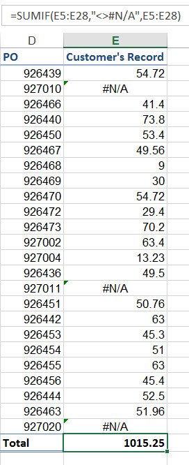
You can use the same function to total a range with #DIV/0! errors as well.
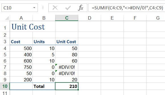
Use this option to replace the errors with a value
Of course if the errors were replaced with a value the SUM function will perform as normal. Let’s look at how to do this for the #DIV/0! error. You can easily do the same for any error that you need to deal with.
In the example below the SUM function isn’t able to display a total due to the errors in the cells within the range.
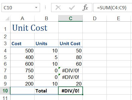
However, if I re-write the ‘Unit Cost’ formula to include the IFERROR function I can replace the #DIV/0! errors with a 0 (zero) value. IFERROR checks if the formula you are using will return an error. If it does it will then replace the error with a value.
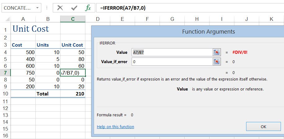
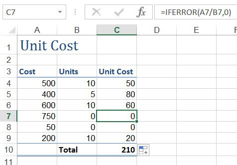
With all cells in the range now holding a value the SUM function held in C10 has an easy time of creating the range total.
We cover VLOOKUP, SUMIF and IFERROR in our very popular Excel Stage 2 and 3 courses. If you are wanting to learn the features of Excel that save you huge amounts of time these courses are definitely for you!
Was this post helpful? Please let us know in the Comments below.


This was a help ! Thanks for complete and brief explanation.
Thanks Tom! So happy our article was helpful to you. Thank you so much for letting us know.
With the SUM function, what formula should I use if I want the cell to show the sum of a range if there are numbers in the range, but to show “NA”, when they are totally no numbers in the range?
Hi there. You can use an IF function. For example, if you were trying to sum the range B6 to B10 this would work =IF(SUM(B6:B10)>0,SUM(B6:B10),”N/A”)
I hope this helps 🙂