Are you are having a few hassles when filtering?

Is the filter not working properly or as you would like it to?

Here are some reasons why your Excel filter may not be working.

Excel has an expectation that you have prepared your data to meet some basic layout standards before you use filter. Get these right and you will minimize filtering hassles.

Check you are following these Filtering rules...

Now only blank rows will be displayed.

You can easily identify the rows as the row number will now be coloured blue.

To delete the blank rows just select them and then right-click over the top of one of the row blue numbers. Select Delete to delete the rows.

Turn filtering off and you will see that the rows have now been removed.

Check your column headings

Check your data has just one row of column headings.

If you need multiple lines for a heading, just type the first line into a cell and then press ALT + ENTER to type on a new line within the cell.

Formatting the cell using Wrap Text also works.

Check for merged cells

Another reason why your Excel filter may not be working may be due to merged cells.

Unmerge any merged cells or so that each row and column has it’s own individual content.

If your column headings are merged, when you filter you may not be able to select items from one of the merged columns.

If you have merged rows, filtering will not pick up all of the merged rows.

Check for errors

Check your data doesn't include errors. For example, if you were trying to filter on the 'Top 10', 'Above Average' or 'Below Average' values in your list (use Number Filters to do this), and error may stop Excel from applying the filter.

To remove errors first use Filter to find them. They are always listed at the bottom of the list so scroll right to the bottom.

If you see one (or many) remove the check mark from ‘(Select All)’ at the top of the list first and then scroll back to the bottom of the list.

Select the error and click OK. Once you have located the error, fix it or delete it and then clear the filter. No go ahead and use Top 10, Above or Below Average and you'll be back in business!

Check for hidden rows

Hidden rows aren’t even shown as a filter option on the filter list.

To unhide rows first select the area containing the hidden rows. This may mean you need to select the row above and below the hidden data.

Then either right-click in the row header area (over the row numbers) and select Unhide or from the Home tab select Format, Hide & Unhide, Unhide Rows.

Extra checks and info...

Check for other filters

Check that a filter hasn't been left on another column.

The best way to clear all of the filters is to click the Clear button on the Ribbon (to the right of the Filter button).

This then leaves Filter turned on, but removes all filter settings allowing you to start again with the full set of your data.

The Filter button is greyed out

If the Filter button is greyed out check that you don't have your worksheets grouped.

You can tell if they are simply by looking at the title bar where the filename is shown at the top of the screen.

If you can see 'Your file name' - Group you currently have worksheets that are grouped.

Just make your way down to one of your worksheets, right-click the sheet tab and then select Ungroup Sheets. The Filter button will now be available 😊

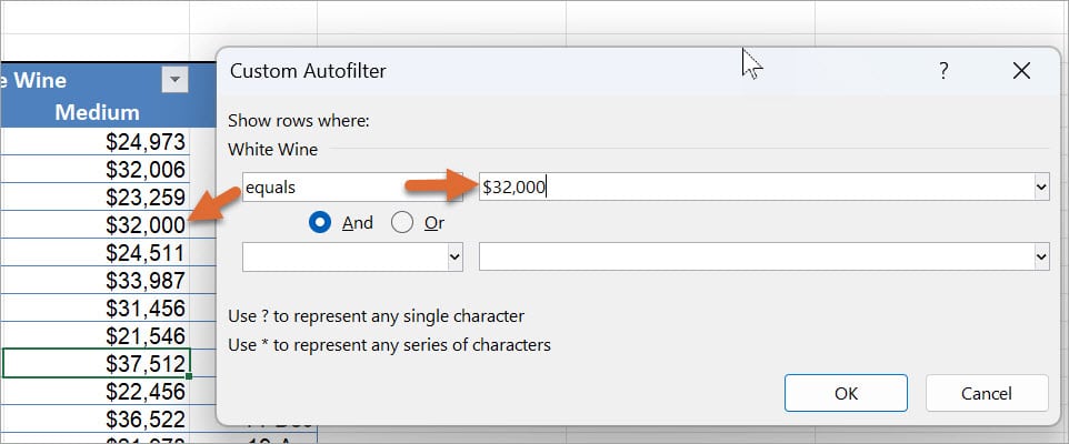
The 'Equals' filter isn't working

If you're using the Number Filter or Date Filter, Equals filter and Excel isn't returning the correct data, check the formats on your data are the same.

For example, if you have 2 cells with 1,000 entered into each and one cell is formatted with the ‘Currency’ format and one with the ‘Number’, when you use the Number Filters, Equals option, Excel will only find matches where you type the format for the number as well.

Just typing 1000 will find a match for the cell formatted with a ‘Number’ format only. Typing $1,000.00 will find the cell formatted as ‘Currency’.

This is the same for dates. 16-Jan-19 will not match 16/01/2019. Therefore, make sure the entire column of data is formatted with the same format to avoid this problem.

 My file is really slow to refresh

If you are finding that your file is starting to become very slow at responding, i.e. the 'whirly-wheel' is displayed for more than a few seconds every time you update your file, check that you only selected the table area before you applied Filter, not entire rows, entire columns or the entire worksheet.

Also, if you have applied Filter to multiple tables within the file you might like to remove Filter from any tables you aren't working with. This may also help eliminate 'whirly-wheel' moments.

I hope one of these tips has seen you back on track again. There are so many reasons why your Excel filter may not be working.

However, these are typically the ones I come across the most so I really hope this blog has helped 😊